Polefigs

Plotting pole figures from EBSD data
Inverse pole figures
Calculating an Orientation Distribution Function from EBSD data

clear all
import_excel_data;

Plotting pole figures from EBSD data

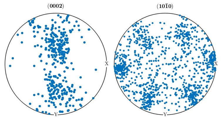
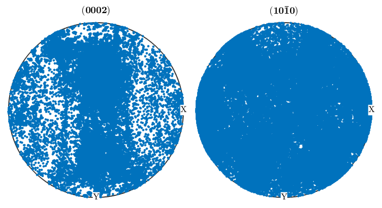
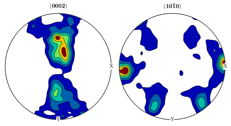
%We can take the orientaion data from an EBSD structure and use it to
%generate pole figures. First, define the crystallographic directions you'd
%like to create pole Figures for, then use the plotPDF command as below:
p1=Miller(0,0,0,2,ebsd('Zirconium').CS);
p2=Miller(1,0,-1,0,ebsd('Zirconium').CS);
figure(1)
plotPDF(ebsd('Zirconium').orientations,[p1 p2])

%The plot we just made will randomly plot a certain number of points from
%the ebsd map onto the pole figure.  If you want to plot all othe points,
%you can do so by setting the 'points' option to 'all'.  It's also useful
%to change the marker size
figure(2)
plotPDF(ebsd('Zirconium').orientations,[p1 p2],'points','all','markerSize',3)

%Having all these points makes it difficult to see what's going on, and
%it's oftentimes more useful to display PF's as contour plots.  The
%contourf option will plot the PF as a filled contour plot, and the option
%after it sets the scale of the contours, in this case from 0 to 6 mrd in
%steps of 1.  If you prefer unfilled plots you can use contour instead of
%contourf

figure(3)
plotPDF(ebsd('Zirconium').orientations,[p1 p2],'contourf',0:1:6)
colorbar;

  I'm plotting 416 random orientations out of 213854 given orientations
  You can specify the the number points by the option "points".
  The option "all" ensures that all data are plotted

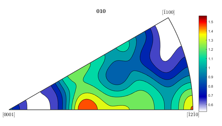
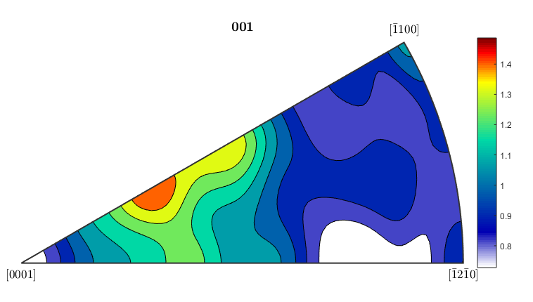
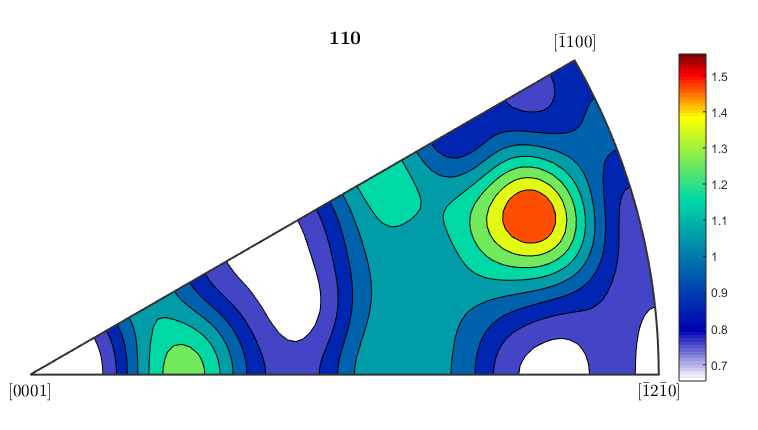
Inverse pole figures

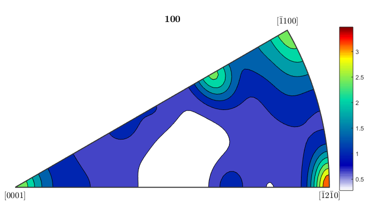
%If you want to plot an inverse pole figure to see which crystal
%orientations are aligned along a given sample direction, MTEX can do it
%quite easily.  The 3 figures below plot inverse pole figures for the
%x,y, and z directions of the ebsd map.  Here we also show that you can
%use mean orientation data from grains instead of considering each
%individual pixel.

[grains,ebsd.grainId,ebsd.mis2mean] = calcGrains(ebsd('indexed'),'angle',5*degree);

figure(1)
plotIPDF(grains(grains.phase==1).meanOrientation,xvector,'contourf')
colorbar;

figure(2)
plotIPDF(grains(grains.phase==1).meanOrientation,yvector,'contourf')
colorbar;

figure(3)
plotIPDF(grains(grains.phase==1).meanOrientation,zvector,'contourf')
colorbar;

%If you want to plot an IPF for an arbitrary direction you can do that as
%well.  The following code will create an IPF for a direction halfway
%between the x and y directions (so going diagonally across the map)

dir=vector3d(1,1,0);
figure(4)
plotIPDF(grains(grains.phase==1).meanOrientation,dir,'contourf')
colorbar;

%All of the figures here were done for the alpha phase, which is phase #1
%in grains.  To get figures for the beta phase, just change the
%(grains.phase==1) to (grains.phase==2).

Calculating an Orientation Distribution Function from EBSD data

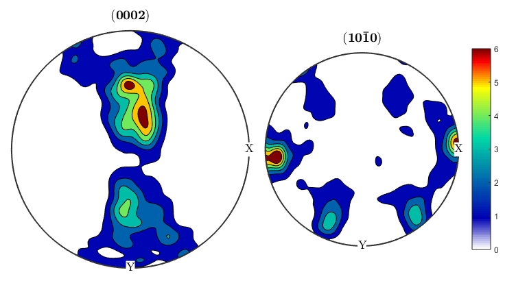
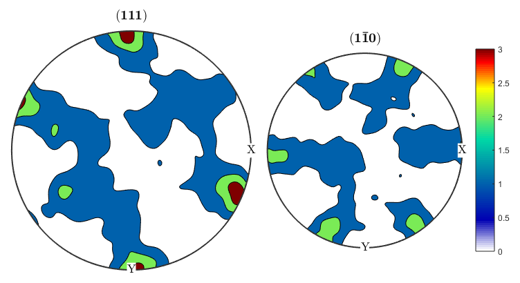
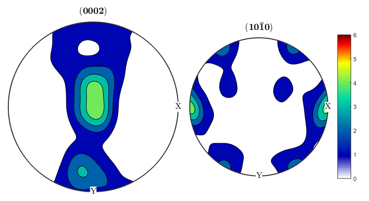
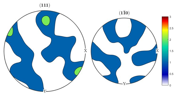
alphaODF=calcODF(ebsd('Zirconium').orientations,'halfwidth',10*degree)

betaODF=calcODF(ebsd('ZirconiumBeta').orientations,'halfwidth',10*degree)

%An ODF contains full information about the distribution of orientations,
%instead of just information about a single crystal direction as in a pole
%figure.

%Let's take another look at the pole figures for our data, this time both
%alpha and beta phasess:

p1=Miller(0,0,0,2,ebsd('Zirconium').CS);
p2=Miller(1,0,-1,0,ebsd('Zirconium').CS);

p1beta=Miller(1,1,1,ebsd('ZirconiumBeta').CS);
p2beta=Miller(1,-1,0,ebsd('ZirconiumBeta').CS);

figure(1)
plotPDF(ebsd('Zirconium').orientations,[p1 p2],'contourf',0:1:6)
colorbar;

figure(2)
plotPDF(ebsd('ZirconiumBeta').orientations,[p1beta p2beta],'contourf',0:1:3)
colorbar;

%It seems like the pole figure is slightly tilted, this is pretty common
%since EBSD samples have to be aligned by hand in the SEM and might be off
%by a few degrees.  We can use an MTEX function on the ODF to corect this.
%The centerSpecimen function takes in an ODF and attempts to find and align
%the sample symmetry.  It returns a rotated ODF along with information
%about the rotation, which I've assigned to the variable tilt.

[cor_alphaODF, rotAlpha]=centerSpecimen(alphaODF);
[cor_betaODF, rotBeta]=centerSpecimen(betaODF);

%We now have corrected ODF's for the alpha and beta phases, as well as the
%rotations applied to them.  Since both are in the same sample, both
%rotations should be the same, so let's check:

rotAlpha

rotBeta

%We can see from the euler angle output of the rotations that they don't
%look like they agree very well. Let's check how much they've been rotated
%by, and the axes about which they're being rotated.

rotAlpha.angle/degree

rotAlpha.axis

rotBeta.angle/degree

rotBeta.axis

%We can see that the alpha phase has been rotated by 25 degrees about an
%axis close to the x axis, while the beta phase is being rotated by 16
%degrees, mostly about the y axis.  It doesn't make physical sense to apply
%two different corrections to the different phases, so we can use the
%rotate() function to rotate one of the ODF's by the correction applied to
%the other.  We can assume that since the sample is mostly alpha, the
%statistics for that phase are better, so let's apply the alpha rotation to
%the beta phase and then plot the results.

figure(3)
plotPDF(cor_alphaODF,[p1 p2],'contourf',0:1:6)
colorbar;

figure(4)
cor_betaODF=rotate(betaODF,rotAlpha);
plotPDF(cor_betaODF,[p1beta p2beta],'contourf',0:1:3)
colorbar;

 
alphaODF = ODF (<a href="matlab:docmethods(alphaODF)">show methods</a>, <a href="matlab:plot(alphaODF)">plot</a>)
  crystal symmetry : Zirconium (6/mmm, X||a*, Y||b, Z||c)
  specimen symmetry: 1
 
  Harmonic portion:
    degree: 28
    weight: 1
 
 
betaODF = ODF (<a href="matlab:docmethods(betaODF)">show methods</a>, <a href="matlab:plot(betaODF)">plot</a>)
  crystal symmetry : ZirconiumBeta (m-3m)
  specimen symmetry: 1
 
  Harmonic portion:
    degree: 28
    weight: 1
 
  searching for a first two fold symmetry axes
  fit: 73%
  fit: 81%
  searching for a second two fold symmetry axes
  fit: 40%
  fit: 40%
  searching for a first two fold symmetry axes
  fit: 5.8%
  fit: 7%
  searching for a second two fold symmetry axes
  fit: -12%
  fit: -12%
 
rotAlpha = rotation (<a href="matlab:docmethods(rotAlpha)">show methods</a>, <a href="matlab:plot(rotAlpha)">plot</a>)
  size: 1 x 1
 
  Bunge Euler angles in degree
     phi1     Phi    phi2    Inv.
  195.759 24.3131 170.364       0
 
 
 
rotBeta = rotation (<a href="matlab:docmethods(rotBeta)">show methods</a>, <a href="matlab:plot(rotBeta)">plot</a>)
  size: 1 x 1
 
  Bunge Euler angles in degree
     phi1     Phi    phi2    Inv.
  273.467  16.099 90.3354       0
 
 

ans =

   25.0610

 
ans = vector3d (<a href="matlab:docmethods(ans)">show methods</a>, <a href="matlab:plot(ans)">plot</a>)
 size: 1 x 1
          x         y         z
  -0.946878 -0.213336  0.240645

ans =

   16.5391

 
ans = vector3d (<a href="matlab:docmethods(ans)">show methods</a>, <a href="matlab:plot(ans)">plot</a>)
 size: 1 x 1
          x         y         z
  0.0266052 -0.973203  0.228405

Contents

Plotting pole figures from EBSD data

Inverse pole figures

Calculating an Orientation Distribution Function from EBSD data