Working_with

Plotting EBSD
Plotting ebsd properties
Grain reconstruction
Grain Reconstruction 2
Combining plots with the hold command
Getting grain statistics
Plotting grain boundaries by angle
Plotting grain boundaries by misorientation axis
Advanced grain boundary analysis
Twin Identification

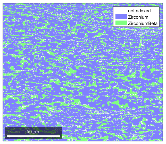
%Ebsd Data is stored in a structure that has many properties
%If you type the name of your ebsd structure, matlab will output a summary
clear all
import_excel_data
ebsd

%Note the names of the various phases are listed.  To select a single phase
%you can specify it by its name or by using conditional indexing to select
%by phased number:

ebsd('Zirconium')

ebsd(ebsd.phase==1)

%though some of the properties are listed, if you want to see a list, type
%in "ebsd." (without quotes) to the command line and press the tab key.
%Matlab will open a list of properties available. This works for most
%structure types in Matlab.  Feel free to experiment with the different
%properties to see what kind of information you can access.

 
ebsd = EBSD (<a href="matlab:docmethods(ebsd)">show methods</a>, <a href="matlab:plot(ebsd)">plot</a>)
 
 Phase  Orientations        Mineral        Color  Symmetry  Crystal reference frame
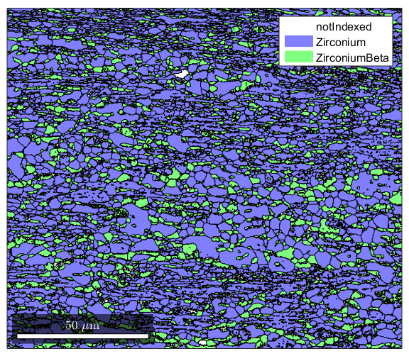
     0    24905 (8%)     notIndexed                                                
     1  213854 (69%)      Zirconium   light blue     6/mmm        X||a*, Y||b, Z||c
     2   71441 (23%)  ZirconiumBeta  light green      m-3m                         
 
 Properties: bands, bc, bs, error, mad, x, y
 Scan unit : um
 
 
ans = EBSD (<a href="matlab:docmethods(ans)">show methods</a>, <a href="matlab:plot(ans)">plot</a>)
 
 Phase   Orientations    Mineral       Color  Symmetry  Crystal reference frame
     1  213854 (100%)  Zirconium  light blue     6/mmm        X||a*, Y||b, Z||c
 
 Properties: bands, bc, bs, error, mad, x, y
 Scan unit : um
 
 
ans = EBSD (<a href="matlab:docmethods(ans)">show methods</a>, <a href="matlab:plot(ans)">plot</a>)
 
 Phase   Orientations    Mineral       Color  Symmetry  Crystal reference frame
     1  213854 (100%)  Zirconium  light blue     6/mmm        X||a*, Y||b, Z||c
 
 Properties: bands, bc, bs, error, mad, x, y
 Scan unit : um

Plotting EBSD

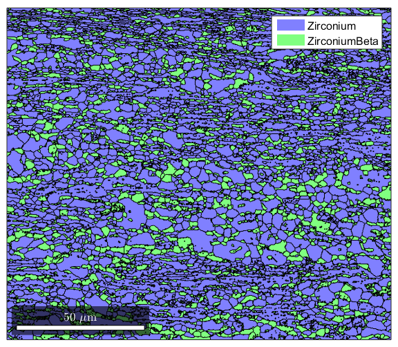
%By default, matlab plots ebsd data by phase (if you have a single phase
%material, this means you won't see much)

plot(ebsd)

Plotting ebsd properties

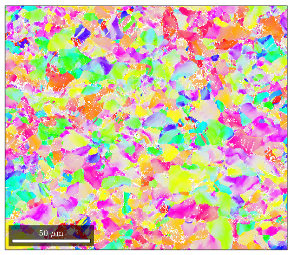
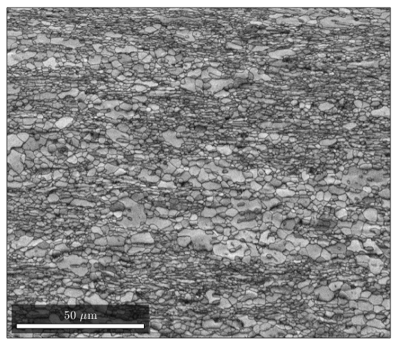
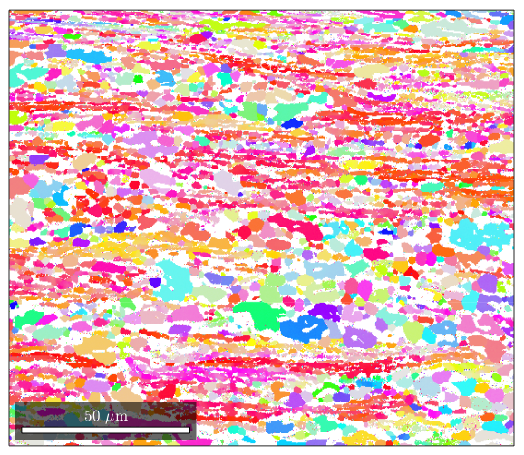
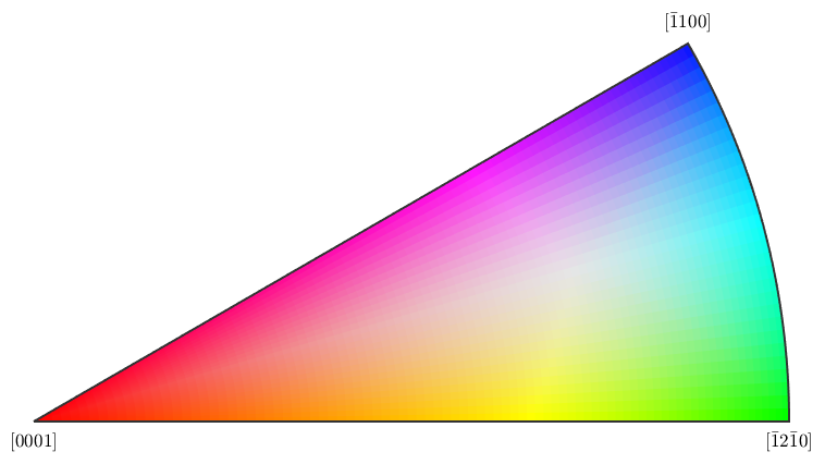
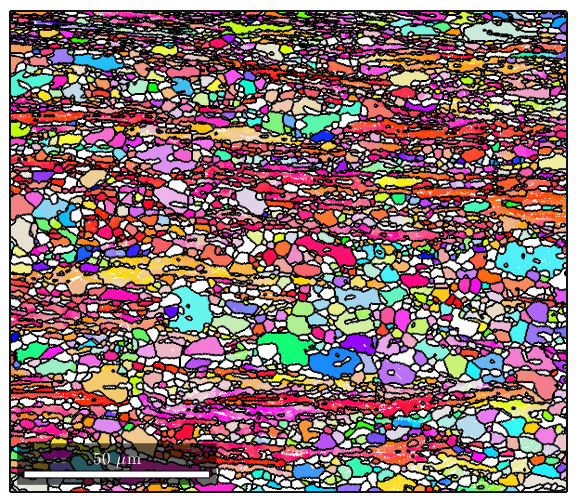
%If you want to plot something else on an EBSD map, you can do so:

%here is a plot of the band contrast
figure(1)
plot(ebsd,ebsd.bc)
colormap('gray');

%We can plot orientations, but only for one phase at a time:
figure(2)
%remember, you can specify a phase within brackets when calling the ebsd structure
plot(ebsd('Zirconium'),ebsd('Zirconium').orientations)

%here is some code that will plot an inverse pole figure showing how the
%colors in figure 2 relate to orientation
figure(3)
oM=ipdfHSVOrientationMapping(ebsd('Zirconium').orientations);
plot(oM)

  I'm going to colorize the orientation data with the 
  standard MTEX colorkey. To view the colorkey do:
 
  oM = ipdfHSVOrientationMapping(ori_variable_name)
  plot(oM)

Grain reconstruction

%MTEX can reconstruct grains from ebsd data.

%calcGrains takes in ebsd and will define a grain boundary as any point
%where there is a change in orientation of 5 degrees or more.  It outputs a
%list of grains, and gives the ebsd structure  new properties called grainId,
%and mis2mean.  GrainId tells which grain each pixel in the map belongs to,
%and mis2mean is the misorientation of each pixel to the mean orientation
%of its grain.
[grains,ebsd.grainId,ebsd.mis2mean] = calcGrains(ebsd,'angle',5*degree);

%We can plot the grains now
figure(1)
plot(grains)

%Note that MTEX has treated non-indexed areas as their own grains.  If
%you'd instead like MTEX to simply absorb non-indexed points into grains
%formed by indexed points, you can issue this command instead (note that
%instead of sending all of ebsd as an argument to calcGrains, we send only
%the indexed parts)

[grains,ebsd.grainId,ebsd.mis2mean] = calcGrains(ebsd('indexed'),'angle',5*degree);

%We can plot the grains now
figure(2)
plot(grains)

Grain Reconstruction 2

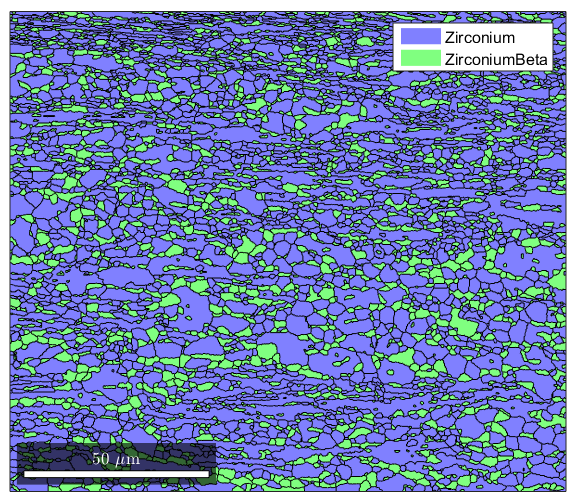
%Often you will see that ther are a lot of reconstructed grains that are
%very tiny, perhaps even a single pixel.  These are usually mis-indexed
%points

[grains,ebsd.grainId,ebsd.mis2mean] = calcGrains(ebsd,'angle',5*degree);

%You can get rid of them and clean up your map a little by first running
%grain reconstruction, then executing the following command to remove any
%points that are in grains less than 3 pixels large:

ebsd(grains(grains.grainSize<3))=[];

%Now we re-run grain reconstruction

[grains,ebsd.grainId,ebsd.mis2mean] = calcGrains(ebsd('indexed'),'angle',5*degree);

%Note that the map of the grains is a lot cleaner now
figure(1)
plot(grains)

Combining plots with the hold command

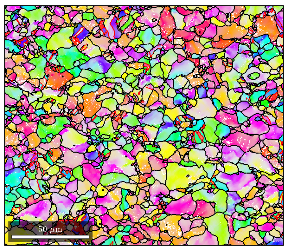
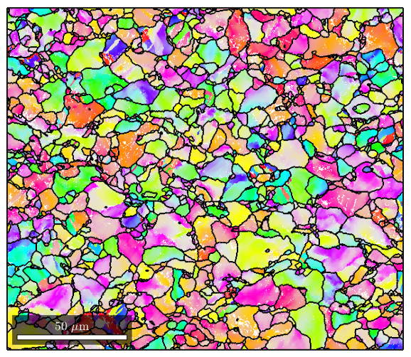
%It's oftentimes useful to combine the raw ebsd data with the reconstructed
%grain boundary data.  Here's an example where we plot the orientation data
%and use matlab's hold feature to add grain boundaries to the figure:

figure(1)
plot(ebsd('Zirconium'),ebsd('Zirconium').orientations);

%now using the hold command we plot a property of grains called boundary.
%This will outline the grain boundaries in black. We'll also set the
%linewidth to 1.5 since the default lines are a bit too thin
hold on
plot(grains.boundary,'linewidth',1.5);
hold off

  I'm going to colorize the orientation data with the 
  standard MTEX colorkey. To view the colorkey do:
 
  oM = ipdfHSVOrientationMapping(ori_variable_name)
  plot(oM)

Getting grain statistics

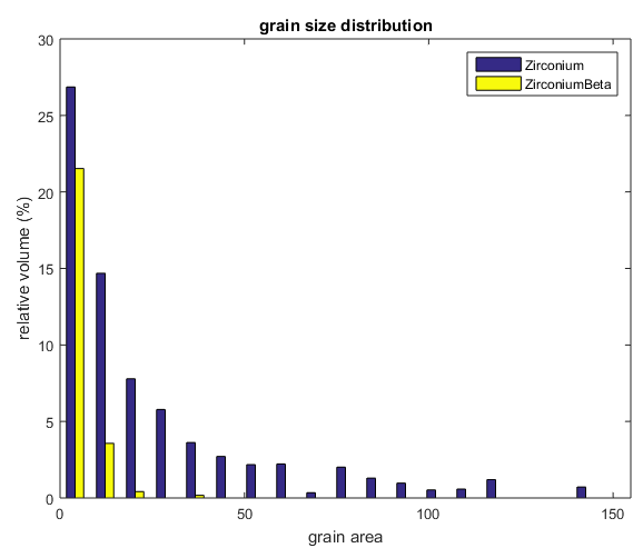
%In MTEX, you can get a histogram of grain sizes by sending your grains
%object to the funciton hist().  The number of bins can also be
%specified.(default is 15)
figure(1)
hist(grains,20)

%You can also use simple matlab functions to get useful information about
%your grains

%Here we calculate the median grain size for all the grains, as well as
%each phase individually. (Note: grains.area returns the area in microns^2,
%and grains.grainSize returns the area in number of pixels.)

median(grains.area)

median(grains(grains.phase==1).area)

median(grains(grains.phase==2).area)

%The grains object has many useful properties! Remember, you can see a list
%of the properties in grains by typing "grains." (without quotes) into the
%Matlab command line and pressing the tab key.

ans =

    1.7709


ans =

    2.5642


ans =

    1.2681

Plotting grain boundaries by angle

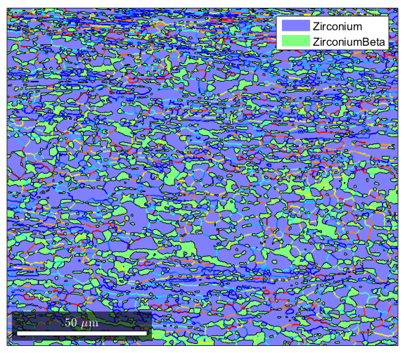
%This gets a little tricky because it takes advantage of the fact that you
%can have multiple "layers" of properties in a single structure

%first we'll define gB as the grain boundary information from grains
gB=grains.boundary;

%Next we define gBAA as the alpha/alpha grain boundaries
gBAA=gB('Zirconium','Zirconium');

%gBBB will be the beta/beta grain boundaries
gBBB=gB('ZirconiumBeta','ZirconiumBeta');

%we now have Matlab plot the grains
plot(grains)

%Using the hold command we plot GBAA nad GBBB and color them by their
%misoreientaiton angle.  This will let us show which grain boundaries are
%high and which are low.  We needed to do this for just the alpha/alpha and
%beta/beta boundaries because MTEX doesn't know how to meaningfully find
%misorientations between diffferent crystal structures
hold on
plot(gBAA,gBAA.misorientation.angle/degree,'linewidth',1.5)
plot(gBBB,gBBB.misorientation.angle/degree,'linewidth',1.5)
hold off

%setting the colormap to 'jet' makes the colorcoding a bit nicer. It's just
%a cosmetic thing.
colormap('jet')

Plotting grain boundaries by misorientation axis

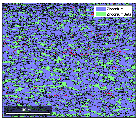
%In addition to the misorientation angle of grain boundaries, it is often
%useful to know which crystallographic direction the misorientation is
%occuring about

%We will define the grain boundaries as in the previous section
gB=grains.boundary;
gBAA=gB('Zirconium','Zirconium');


%Now we define an axis that we are interested in.  We define axisA as the
%{10-10} plane normal. The last argument is the crystal symmetry for the
%phase in question, which must be provided so MTEX knows what kind of
%structure your Miller variable goes with

axisA=Miller(1,0,-1,0,ebsd('Zirconium').CS);


%Now, we find which boundaries have a mistorientation axis close to the
%ones we've defined. We define axisGBA  as a conditional
%statement, so we can use it for conditional indexing.  The line below
%will find all grain boundaries that have a misorientation axis within 2
%degrees of the one we defined.

axisGBA=angle(gBAA.misorientation.axis,axisA)<5*degree;

%Here we plot the grains, then use the hold command to add the special
%grain boundaries we're interested in.  The alpha/alpha grains with their
%{10-10} misorientation axis
plot(grains)
hold on
plot(gBAA(axisGBA),'linecolor','red','linewidth',1.5);
hold off

Advanced grain boundary analysis

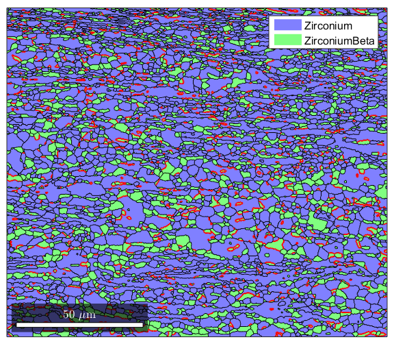
%This section will show how to pick out very specific grain boundaries
%where both the misorientation axis and angle are defined.  This can be
%used for twin identification, which will be shown in another section, but
%here we will use it to look at the Burgers relationship between the alpha
%and beta phase.

%We start by defining 4 Miller directions, such that a1//b1 and a2//b2.
%This will let us define the orienation relationship betweeen alpha and
%beta phases
a1=Miller(0,0,0,2,ebsd('Zirconium').CS);
b1=Miller(1,1,0,ebsd('ZirconiumBeta').CS);
a2=Miller(1,1,-2,0,ebsd('Zirconium').CS);
b2=Miller(1,1,1,ebsd('ZirconiumBeta').CS);

%Next, we create an orientation map from alpha to beta based on the sets of
%parallel directions we just defined.
ab=orientation('map',a1,b1,a2,b2,ebsd('Zirconium').CS,ebsd('ZirconiumBeta').CS);

%We we now want to get just the grain boundaries that are alpha/beta
%boundaries

gBAB=grains.boundary('Zirconium','ZirconiumBeta');

%Now we will take all alpha/beta boundaries that have a misorientation
%within 5 degrees of the relationship we defined
isBurgers=angle(gBAB.misorientation,ab)<5*degree;

%Finally, we plot the results using conditional indexing:

plot(grains);
hold on
plot(gBAB(isBurgers),'linecolor','red','linewidth',1.5);
hold off

Twin Identification

clear all
%Twins in Zr and other materials, we sometimes see a lot of twins formed
%during deformation.  It's really easy to pick out twins from EBSD data
%with MTEX. The MTEX help page on this is actually pretty good:
% http://mtex-toolbox.github.io/files/doc/TwinningAnalysis.html

%First we'll import a dataset from a tensile sample that has been heavily
%deformed
import_increment3;
figure(1)
plot(ebsd('Zirconium'),ebsd('Zirconium').orientations);

%Now run grain reconstruction.  This map has some poorly indexed points, so
%we'll get rid of any grains smaller than 3 pixels.
[grains,ebsd.grainId,ebsd.mis2mean] = calcGrains(ebsd('indexed'),'angle',5*degree);

ebsd(grains(grains.grainSize<3))=[];

[grains,ebsd.grainId,ebsd.mis2mean] = calcGrains(ebsd('indexed'),'angle',5*degree);

%Now we pick out the Zr/Zr grain boundaries:

bounds=grains.boundary;

boundsZr=bounds('Zirconium','Zirconium');

%Now we define the twinning orientation relationship.  In Zr the
%relationship is as defined below, where t1//t2 and t3//t4
t1=Miller(1,1,-2,0,ebsd('Zirconium').CS);
t2=Miller(2,-1,-1,0,ebsd('Zirconium').CS);
t3=Miller(-1,0,1,1,ebsd('Zirconium').CS);
t4=Miller(1,0,-1,1,ebsd('Zirconium').CS);

twinning = orientation('map',t1,t2,t3,t4)

%Now we check which grain boundaries are twins by setting a condition to
%check if the boundary's mistorientation is within 5 degrees of the
%orientation relationship, then use conditional indexing:

istwinning=angle(twinning,boundsZr.misorientation)<5*degree;
twinboundaries=boundsZr(istwinning);

%Now plot the data, using the hold command to
%plot the normal boundaries in black and the twin boundaries overtop in red.
figure(2)
plot(ebsd('Zirconium'),ebsd('Zirconium').orientations)

hold on
plot(grains.boundary,'linewidth',1.5);
plot(twinboundaries,'linewidth',1.5,'linecolor','red');
hold off

%If you like, there's a command to merge twins with their parents, so that
%they will be considered a single grain:

[mergedGrains,parentId] = merge(grains,twinboundaries);

%Now we can plot our merged grain boundaries over the data:
figure(3)
plot(ebsd('Zirconium'),ebsd('Zirconium').orientations)

hold on
plot(mergedGrains.boundary,'linewidth',1.5);
hold off

%This also lets you see what your untwinned grain size looks like:

median(grains.area)

median(mergedGrains.area)

%Finally, you can get the twin area fraction like this.  First we get the
%grain id numbers of all the twins.  The unique() function makes sure
%there's no duplicates.

twinId = unique(boundsZr(istwinning).grainId);

% Next we ge the sum of all the twins, and divide them from the sum of the
% areas of the entire set of grains
twinFraction=sum(area(grains(twinId))) / sum(area(grains)) * 100

  I'm going to colorize the orientation data with the 
  standard MTEX colorkey. To view the colorkey do:
 
  oM = ipdfHSVOrientationMapping(ori_variable_name)
  plot(oM)
 
twinning = misorientation (<a href="matlab:docmethods(twinning)">show methods</a>, <a href="matlab:plot(twinning)">plot</a>)
  size: 1 x 1
  crystal symmetry : Zirconium (6/mmm, X||a*, Y||b, Z||c)
  crystal symmetry : Zirconium (6/mmm, X||a*, Y||b, Z||c)
 
  Bunge Euler angles in degree
  phi1     Phi    phi2    Inv.
   330 94.7957     330       0
 
 
  I'm going to colorize the orientation data with the 
  standard MTEX colorkey. To view the colorkey do:
 
  oM = ipdfHSVOrientationMapping(ori_variable_name)
  plot(oM)
  I'm going to colorize the orientation data with the 
  standard MTEX colorkey. To view the colorkey do:
 
  oM = ipdfHSVOrientationMapping(ori_variable_name)
  plot(oM)

ans =

    2.3553


ans =

    2.5126


twinFraction =

   14.7671

Contents

Plotting EBSD

Plotting ebsd properties

Grain reconstruction

Grain Reconstruction 2

Combining plots with the hold command

Getting grain statistics

Plotting grain boundaries by angle

Plotting grain boundaries by misorientation axis

Advanced grain boundary analysis

Twin Identification